refer to: https://f1tenth.org/course.html

Introduction

In the rapidly evolving field of autonomous vehicles, simulators like F1Tenth play a crucial role in the development and testing of advanced control algorithms. This report details the implementation and evaluation of several key algorithms within the F1Tenth simulator, aimed at enhancing the autonomous navigation capabilities of the simulated vehicles. The algorithms covered in this report include Wall Following, Follow the Gap, Scan Matching, Pure Pursuit, Hector SLAM, and PEB Path Planning.

1. Wall Following

The wall-following algorithm aims to keep the vehicle at a consistent distance from the nearest wall (left or right wall) to achieve stable and reliable navigation in corridor-like environments. The algorithm uses a lidar sensor to measure the distance to the wall and adjusts the steering angle to maintain the desired set path to ensure smooth driving along the wall. The overall control strategy uses PID control.

The general equation for a PID controller in the time domain:
$$
u(t) = K_p e(t) + K_i \int_0^t e(t’) , dt’ + K_d \frac{d}{dt} e(t)
$$
A PID controller is a way to maintain certain parameters of a system around a specified set point. PID controllers are used in a variety of applications requiring closed-loop control, such as in the VESC speed controller on your car.

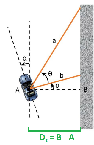
In the context of our car, the desired distance to the wall should be our set point for our controller, which means our error is the difference between the desired and actual distance to the wall. This raises an important question: how do we measure the distance to the wall, and at what point in time? One option would simply be to consider the distance to the right wall at the current time (let’s call it Dt). Let’s consider a generic orientation of the car with respect to the right wall and suppose the angle between the car’s x-axis and the axis in the direction along the wall is denoted by α. We will obtain two laser scans (distances) to the wall: one 90 degrees to the right of the car’s x-axis (beam b in the figure), and one (beam a) at an angle θ ( 0< θ ≤70 degrees) to the first beam. Suppose these two laser scans return distances a and b, respectively.

we can express α as:
$$
α=tan^{-1}(\frac{acos(θ)-b}{asin(θ)})
$$
We can then express 𝐷𝑡 as:
$$
D_t=bcos(α)
$$

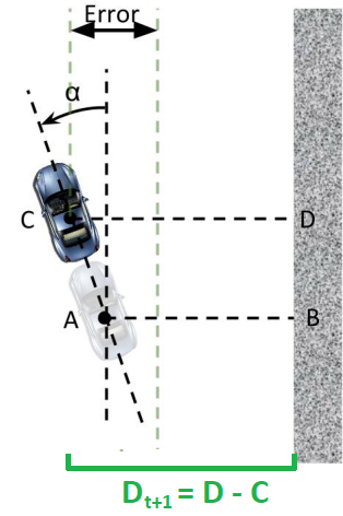
However, we have a problem on our hands. Remember that this is a race: your car will be traveling at a high speed and therefore will have a non-instantaneous response to whatever speed and servo control you give to it. If we simply use the current distance to the wall, we might end up turning too late, and the car may crash. Therefore, we must look to the future and project the car ahead by a certain lookahead distance (let’s call it 𝐿). Our new distance 𝐷𝑡+1 will then be:
$$
D_{t+1}=D_t+Lsin(α)
$$

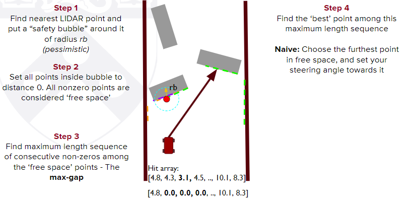
2. Follow the Gap

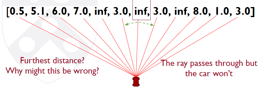
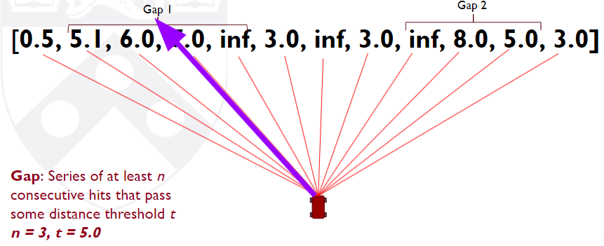
Follow the Gap is a reactive navigation strategy that identifies the largest ‘gap’ in a field of obstacles and directs the vehicle through it. This method is particularly useful in cluttered environments, where traditional path planning methods might struggle. The algorithm processes LIDAR data to detect open spaces, dynamically adjusting the vehicle’s trajectory to navigate through these gaps safely.

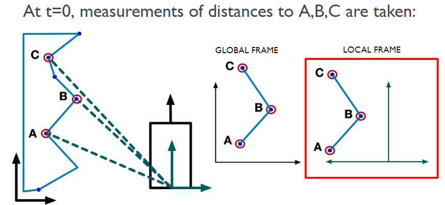
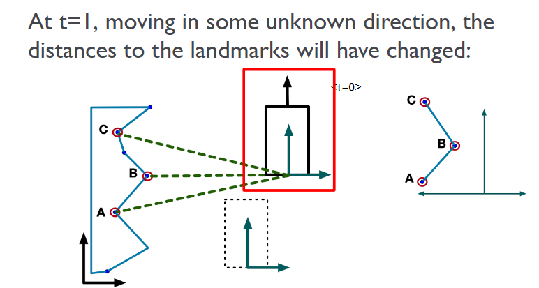
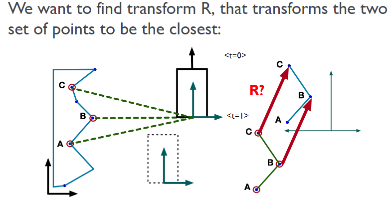
3. Scan Matching

Scan Matching involves comparing the current scan from LIDAR sensors with a previously known map to determine the vehicle’s position. This algorithm is integral to accurate localization, which is crucial for consistent performance in environments with complex geometries. By continuously updating the vehicle’s position and orientation, scan matching enhances the overall stability and reliability of the navigation system.

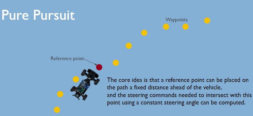
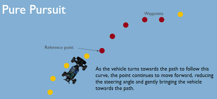
4. Pure Pursuit

Pure Pursuit is a path tracking algorithm that computes the necessary steering commands to follow a predefined path. The algorithm uses a ‘look-ahead’ point on the desired path and calculates the curvature that will guide the vehicle to this point. This approach is straightforward yet effective, making it widely used in the field of autonomous driving.

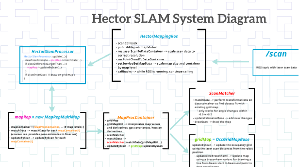
5. Hector SLAM

Hector SLAM (Simultaneous Localization and Mapping) is an algorithm that builds a map of the environment while simultaneously keeping track of the vehicle’s location within it. Unlike other SLAM techniques, Hector SLAM can perform well in environments lacking distinctive features and does not require odometry data, making it well-suited for vehicles equipped solely with LIDAR.

6. PEB Path Planning

PEB (Predict, Evaluate, Build) Path Planning is an advanced algorithm that anticipates potential paths, evaluates them based on a set of predefined criteria, and then selects the most optimal route. This method not only considers the immediate path but also anticipates future obstacles, effectively enhancing navigational decisions in dynamic environments.

Predict:

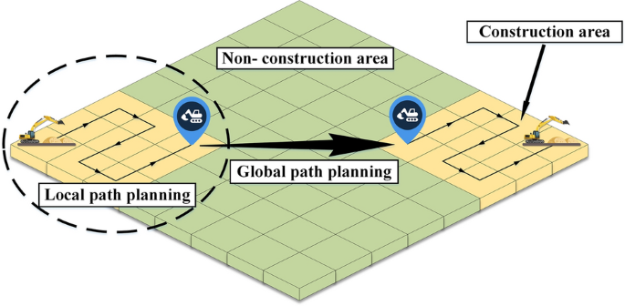
• In the scenario shown, the algorithm predicts paths that account for both static obstacles (like the designated construction area) and dynamic changes (such as potential movement within the non-construction area). This prediction would use sensor inputs and pre-existing map data to identify feasible paths.
• The Global Path Planning arrow shows a broad route that the vehicle intends to follow, bypassing major obstacles and spanning the entire map from one end to the other.

Evaluate:

• Once potential paths are predicted, the algorithm evaluates them based on criteria such as safety, efficiency, and feasibility. This step might involve computational models to simulate the travel time, fuel or energy consumption, and risk of encountering obstacles or entering restricted zones.
• The evaluation might also differentiate between paths that cross higher-risk areas like construction zones and those that stay within safer, non-construction zones. Paths might be ranked or scored based on these evaluations.

Build:

• After evaluating the different paths, the algorithm builds or selects the optimal path for navigation. This step includes the integration of the global path plan with more responsive Local Path Planning to handle immediate obstacles or changes in the environment that weren’t accounted for in the global path.
• The local path planning indicated in the image shows more immediate, reactive navigation choices, adjusting the vehicle’s course in real time to adapt to ground-level variables and shorter-range obstacles or requirements.